Next: Fitting with Stochastic Gradient Up: Regularized Logistic Regression Previous: Logistic Regression Model
The maximum a posteriori (MAP) estimates of parameters are defined to
be the parameters that minimize the error function. The error
function for parameters ![]() under logistic regression with Laplace
priors consists of a likelihood component and a prior component. The
likelihood error is the negative log likelihood of the training labels
given the training data and parameters. The prior component is the
log likelihood of the parameters in the prior.
under logistic regression with Laplace
priors consists of a likelihood component and a prior component. The
likelihood error is the negative log likelihood of the training labels
given the training data and parameters. The prior component is the
log likelihood of the parameters in the prior.
We used Laplace priors with means of zero and variances ![]() which
varied by task. The intercept is assumed to be the first feature (position
0) and is always given a noninformative prior
(equivalently a Laplace prior with infinite variance,
which
varied by task. The intercept is assumed to be the first feature (position
0) and is always given a noninformative prior
(equivalently a Laplace prior with infinite variance,
![]() ). Each feature is given the same prior variance.
). Each feature is given the same prior variance.
The Laplace prior (equivalently regularization or shrinkage with the
![]() norm, also known as the lasso) enforces a preference for
parameters that are zero, but otherwise is more dispersed than a
Gaussian prior (equivalently regularization or shrinkage with the
norm, also known as the lasso) enforces a preference for
parameters that are zero, but otherwise is more dispersed than a
Gaussian prior (equivalently regularization or shrinkage with the
![]() norm, also known as ridge regression). A number of experiments
in natural language classification have shown the Laplace prior to be
much more robust and accurate under cross-validation than either
maximum likelihood estimation or the more common Gaussian prior
[Genkin et al., Goodman 03].
norm, also known as ridge regression). A number of experiments
in natural language classification have shown the Laplace prior to be
much more robust and accurate under cross-validation than either
maximum likelihood estimation or the more common Gaussian prior
[Genkin et al., Goodman 03].
Given a sequence of ![]() data points
data points
![]() ,
with
,
with
![]() and
and
![]() ,
the log likelihood of the data in a model with parameter
matrix
,
the log likelihood of the data in a model with parameter
matrix ![]() is:
is:
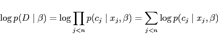 |
(4) |
A Laplace, or double-exponential, prior with zero means and diagonal
covariance is specified by a variance parameter ![]() for each
dimension
for each
dimension ![]() . The prior density for the full parameter matrix
is:
. The prior density for the full parameter matrix
is:
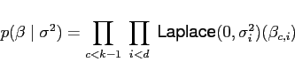 |
(5) |
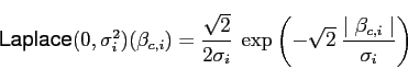 |
(6) |
The Laplace prior has fatter tails than the Gaussian, and is also more concentrated around zero. Thus it is more likely to shrink a coefficient to zero than the Gaussian, while also being more lenient in allowing larger coefficients.
The full error function is the sum of the log likelihood and log prior
given parameters ![]() , training data
, training data ![]() and prior variance
and prior variance ![]() :
:
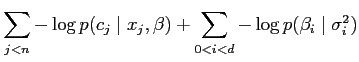 |
This error function is concave and thus has a unique minimum, which is the MAP es4timate.