We can now use the imputed profit vector ![]() at any time
at any time ![]() in order to make
a choice from the
set of efficient points.
For example, given
in order to make
a choice from the
set of efficient points.
For example, given ![]() competing quantizers
competing quantizers
![]() , let
, let ![]() be a set of allocation processes holding Axiom 1 through Axiom 4.
From Axiom 1 and Axiom 3 we have that
be a set of allocation processes holding Axiom 1 through Axiom 4.
From Axiom 1 and Axiom 3 we have that ![]() is a convex set of allocation processes. Hence, by Theorem 1, the concept of ``efficient allocation process''
is a convex set of allocation processes. Hence, by Theorem 1, the concept of ``efficient allocation process'' ![]() is now characterized by profit maximization. That is, maximization of
is now characterized by profit maximization. That is, maximization of ![]() with respect to
with respect to ![]() over the set of allocation processes
over the set of allocation processes ![]() at any given time
at any given time ![]() . Given that
. Given that ![]() is a compact set (by Axiom 1 and Axiom 3),
the existence of solution for this maximization problem is guaranteed by the Weierstrass Theorem since the inner product
is a compact set (by Axiom 1 and Axiom 3),
the existence of solution for this maximization problem is guaranteed by the Weierstrass Theorem since the inner product ![]() is a continuous function.
is a continuous function.
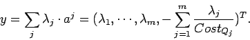
From Axiom 1 we have that
![\begin{displaymath}y = A \cdot \lambda = [a^1, a^2, \cdots, a^m] \cdot \left( \b...
...lambda_m
\end{array} \right) = \sum_{j} \lambda_j \cdot a^j
\end{displaymath}](img34.png)
Since
![]() we then have that
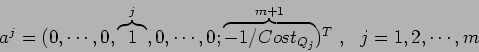
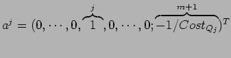
we then have that ![]() assigns
assigns ![]() bits to quantizer
bits to quantizer ![]() ,
,
![]() , with a total bit consumption of
, with a total bit consumption of
![]() , assuming
, assuming
 :
:
Then, it follows that the bit allocation set ![]()
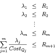
Then the problem of finding
![]() which maximizes
which maximizes
 ,
subject to the constraints
,
subject to the constraints
We shall consider an example of these problems. It solves the bit allocation analysis among three quantizers
![]() at a certain time
at a certain time ![]() . We have that the respective cost of quantization
. We have that the respective cost of quantization ![]() for each quantizer
for each quantizer ![]() is:
is:
![]() bpp;
bpp;
![]() bpp; and
bpp; and
![]() bpp.
bpp.
The three basic allocation processes are (Table I):
![\begin{displaymath}
y = [a^1, a^2, a^3] \cdot \left( \begin{array}{c}
\lambda_1...
...( \begin{array}{c} 144 \\ 0 \\ 31 \\ - 782 \end{array} \right)
\end{displaymath}](img114.png) |
(4) |
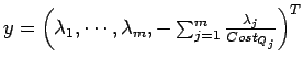
For this example we assume that the imputed profit vector ![]() is
is
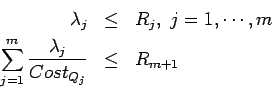
For this example the bit allocation analysis can be represented by:
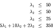
By Theorem 1, the efficient combination of allocations up to the bit resource limitation at this time is the solution of this linear programming problem (where ![]() represents the efficient allocation for quantizer
represents the efficient allocation for quantizer ![]() ): (i)
): (i)
![]() bits; (ii)
bits; (ii)
![]() bits; and (iii)
bits; and (iii)
![]() bits.
No desired bit allocation for a particular quantizer can be increased without decreasing other desired quantizer allocation or increasing bit consumption, at the given profit vector.
bits.
No desired bit allocation for a particular quantizer can be increased without decreasing other desired quantizer allocation or increasing bit consumption, at the given profit vector.